Working of Forecasting in Analytics Plus
Analytics Plus offers a powerful forecasting engine that employs various techniques to analyze your data, identify patterns and predict future values accurately. The forecasting engine offers a range of customization such as the forecasting mode, number of units to be forecasted, number of data points to be ignored in the past data and the type of formatting to be applied over the forecasted data points.
- Supported data series
- Selecting the forecasting model
- Verifying the selected forecasting model
- Forecasting data
Supported data series
Analytics Plus allows you apply forecasting over a report that has at least one aggregate column plotted over a continuous time series data (data that is collected at equal time intervals). The forecasting engine requires a minimum of six continuous data points in the time series to analyze and forecast data accurately. A higher number of data points will increase the accuracy of your data forecasts.
In case there are missing values in your data, Analytics Plus will automatically fill values for the missing data points using the least most recurrent interval. If more than 40% of the values are missing, forecasting will not be possible.
Note: To ensure accurate forecasts, ensure that the number of forecasted values is not greater than 40% of the available data points, i.e., if 10 data points are available in a data series, forecast up to 4 data points for accurate results.
Selecting the forecasting model
By leveraging the patterns identified in the time series data, the forecasting engine initially picks out a set of forecasting models. The model that provides the best result for your data will then be selected as the forecasting model for your specific data series.
The following are the forecasting models available in Analytics Plus. Each of these models has several sub-categories.
You can choose to select the model you require, or allow Analytics Plus to automatically compute the forecasting model that is best suited for your data.
Regression
Regression analyses the behavior of the data series to identify the relationship between various values. On establishing patterns, different regression models such as linear, logarithmic, exponential, power and polynomial (up to the 7th degree) will be computed. These models will each plot an output, and the final model will be identified by calculating the R squared value (or the coefficient of determination). The model with the highest R squared value is selected as the regression model that is best suited for the data series.
Seasonality Trend Loess Decomposition (STL)
This model utilizes the trend, seasonality and error (or randomness) components to compute future data points. On identifying the three components in your data series, the STL model will utilize one of two methods to calculate the future values.
Identifying the trend, seasonality and randomness
To select the STL model that is best suited for your data, the presence of trend, seasonality and randomness in the time series data needs to be identified.
Trend: It refers to a uniform increase or decrease in a series over time. The forecasting engine detects the presence of trends using the Regression model. If the line drawn using the Regression model is straight, there is no trend in the data series. However, if the line drawn has a slope, it indicates the presence of a trend in the data series.
Seasonality: It is a common pattern that repeats in regular intervals in the data series, and is calculated using spectral analysis.
Randomness: Randomness or error refers to the random points in the data series that do not have any identified pattern among the data series.
Based on the three components, future values will be calculated using either the additive or multiplicative model. The additive model will add the trend, seasonality and randomness, while the multiplicative model will multiply the three components.
Additive model: In this model, the contributions of the components in a time series (trend, seasonality and error) are almost the same.
Multiplicative model: In a multiplicative model, the trend and seasonality components will be multiplied with each other, and added to the error component.
The STL model that is best suited for the data series will be identified by calculating the Root Mean Square Error (RMSE) value. The Seasonality Trend Loess Decomposition model also accounts for smoothing random points.
Exponential Smoothing Technique (ETS)
In the ETS model, the forecasted values are a weighted sum of past observations, with an exponentially decreasing weight for the past observations. Therefore, recent values in the data series will hold a higher influence over the forecasted values. The Exponential Smoothing Technique model is thereby best suited when recent values are more important for calculating future data points.
The forecasting engine in Analytics Plus provides a variety of exponential smoothing techniques, for different types of time series data. The following image illustrates the various combinations of the different trend and seasonality components that result in ETS models.
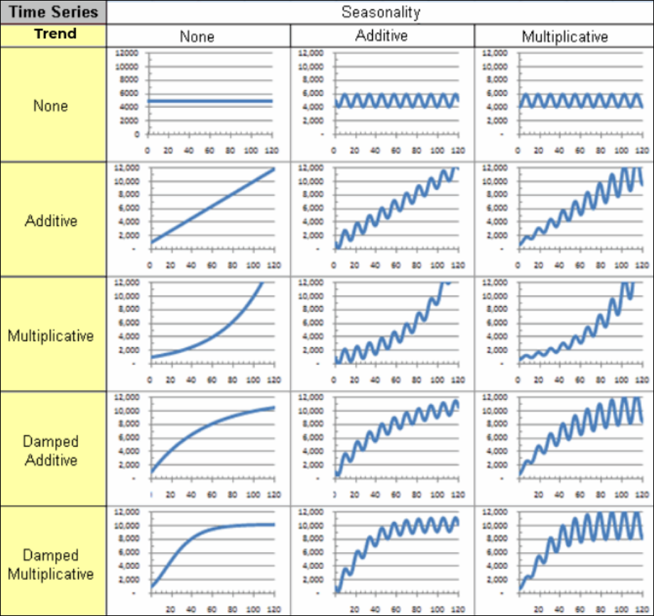
Several smoothing parameters are required while forecasting data using the ETS models. These parameters are listed below:
Alpha: Known as the smoothing factor or the smoothing co-efficient for level, this parameter controls the rate at which the influence of the past values exponentially decay. This value should be between 0 and 1.
Beta: This is the smoothing factor for trend, and it controls the influence of the trend component. This value should be between 0 and 1.
Gamma: It is the smoothing parameter for seasonality, and controls the influence of the seasonal component. This value should be between 0 and 1.
Phi: Known as the damping co-efficient, it is used to control the rate of dampening and smoothen the graph. This value should be between 0 and 1.
Frequency: This depicts the total number of data points it takes before seasonality occurs, i.e., before the seasonal pattern is repeated. This value can range from 2, to an upper limit of half the number of data points available.
You can either choose to select the Exponential Smoothing Technique model you require, or the ETS model that is best suited for your data series will be identified automatically, using the Akaike information criterion (AIC) method.
Autoregressive Integrated Moving Average (ARIMA)
This is a conventional approach to time series modeling that relies on successive transformations until white noise or the original signal of the underlying data generation process is extracted. It employs auto-regression processes and moving averages to propagate the nature of the series, along with probable errors. The ARIMA model is best suited for a random data series, with no proper trend and seasonality components.
The following are the various parameters that are involved in forecasting data using the ARIMA model:
Auto-regressive order (p): This parameter denotes the number of auto-regressive terms in the data series.
Moving average order (q): This parameter indicates the number of previous error values that are accounted for each moment in the time series.
Integration order (d): It represents the number of times a data point has to be differentiated to result in a stationary signal (i.e. a signal that has a constant mean over time).
Frequency: This parameter depicts the seasonality profile generated using spectral analysis, and is used to remove repetitive effects.
Verifying the selected forecasting model
The forecasting engine will compare the results from the various models, and identify the best one to forecast your chart using the Akaike information criterion (AIC). In cases where two models provide similar results at the end of this computation, the Bayesian information criterion (BIC) method will be employed to select the final forecasting model that is best suited for the data series.
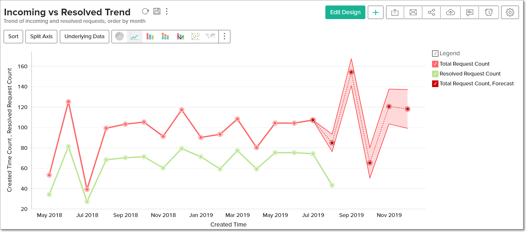
Forecasting data
Based on these calculations, Analytics Plus will use the most-suited forecasting model and generate the future data points for your data series.