Your pg_stat_statements report shows a query climbing from 12ms to 340ms average execution time, but your monitoring dashboard just says "database latency increased." You're left manually cross-referencing slow query logs, checking connection pool exhaustion, and guessing whether you're looking at memory pressure, a rogue index scan, or a transaction holding row locks during peak traffic. The metrics flagged a problem. They didn't explain why it happened.
That causal chain, from architectural decisions to observable failure modes, is what this guide covers. Understanding which components degrade under which conditions makes your monitoring decisions defensible at 2am on a Saturday.
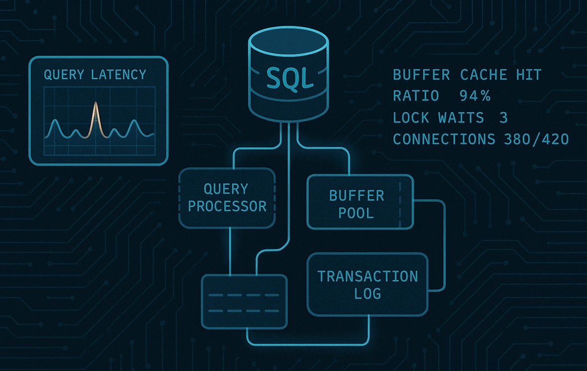
SQL database architecture: the components that actually matter
Every SQL database, whether MySQL 8.0, PostgreSQL 16, or SQL Server 2022, shares four core components. The query processor handles parsing, optimization, and execution. The storage engine manages how data is physically read from and written to disk. The transaction log ( WAL in PostgreSQL, redo log in MySQL InnoDB) records changes before they're committed to storage. The buffer pool caches data pages in memory to reduce disk I/O.
What breaks under load is predictable once you understand what each component actually does at runtime.
The query processor's optimizer generates an execution plan based on table statistics. When those statistics are stale (after a large batch import, for example), the optimizer picks a suboptimal plan. A table with 10 million rows where the statistics still reflect 500,000 gets a full sequential scan when an index seek would have sufficed. The execution cost multiplies by orders of magnitude, and all you see from the outside is latency.
Most deployments undersize the buffer pool, making it a frequently misconfigured bottleneck in mid-sized systems. PostgreSQL's shared_buffers defaults to 128MB, adequate for a development instance and inadequate for a production system with 50GB of hot data. Changing shared_buffers requires a PostgreSQL service restart, and you should update effective\_cache\_size alongside it so the planner accounts for OS page cache as well. Note that gains from shared_buffers diminish above 8-10GB on hosts with more than 32GB of RAM. MySQL InnoDB's innodb\_buffer\_pool_size serves the same role and defaults to 128MB as well, though it can be resized dynamically since MySQL 5.7. SQL Server manages its buffer pool automatically but caps it through the max server memory setting. Regardless of engine, when the working set exceeds buffer pool capacity, every cache miss translates to a disk read. On spinning disks, that's 10-15ms per read for typical 7,200 RPM drives (5-7ms on high-performance 15,000 RPM enterprise drives). On SSDs, latency depends on interface: NVMe drives reach as low as 25 microseconds, while SATA SSDs are closer to 175 microseconds, both orders of magnitude faster than spinning media but still far slower than sub-microsecond memory access. At 10,000 queries per second, that difference in read latency compounds fast.
Write-ahead logging is a durability guarantee. Every major engine implements it: PostgreSQL writes changes to WAL before acknowledging a commit, MySQL InnoDB writes to its redo log, and SQL Server writes to its transaction log. In each case, fsync latency on your storage device directly affects write transaction throughput. If your log directory sits on the same volume as your data directory and that volume is under I/O pressure, transaction commit times spike even when query execution time looks normal.
When a query arrives, execution runs through parser validation, optimizer plan selection, and executor against the buffer pool, then (on cache miss) disk read back into the buffer pool. Write operations go to the transaction log first, then to the storage engine. Monitoring any single point in this chain without the others produces incomplete signal.
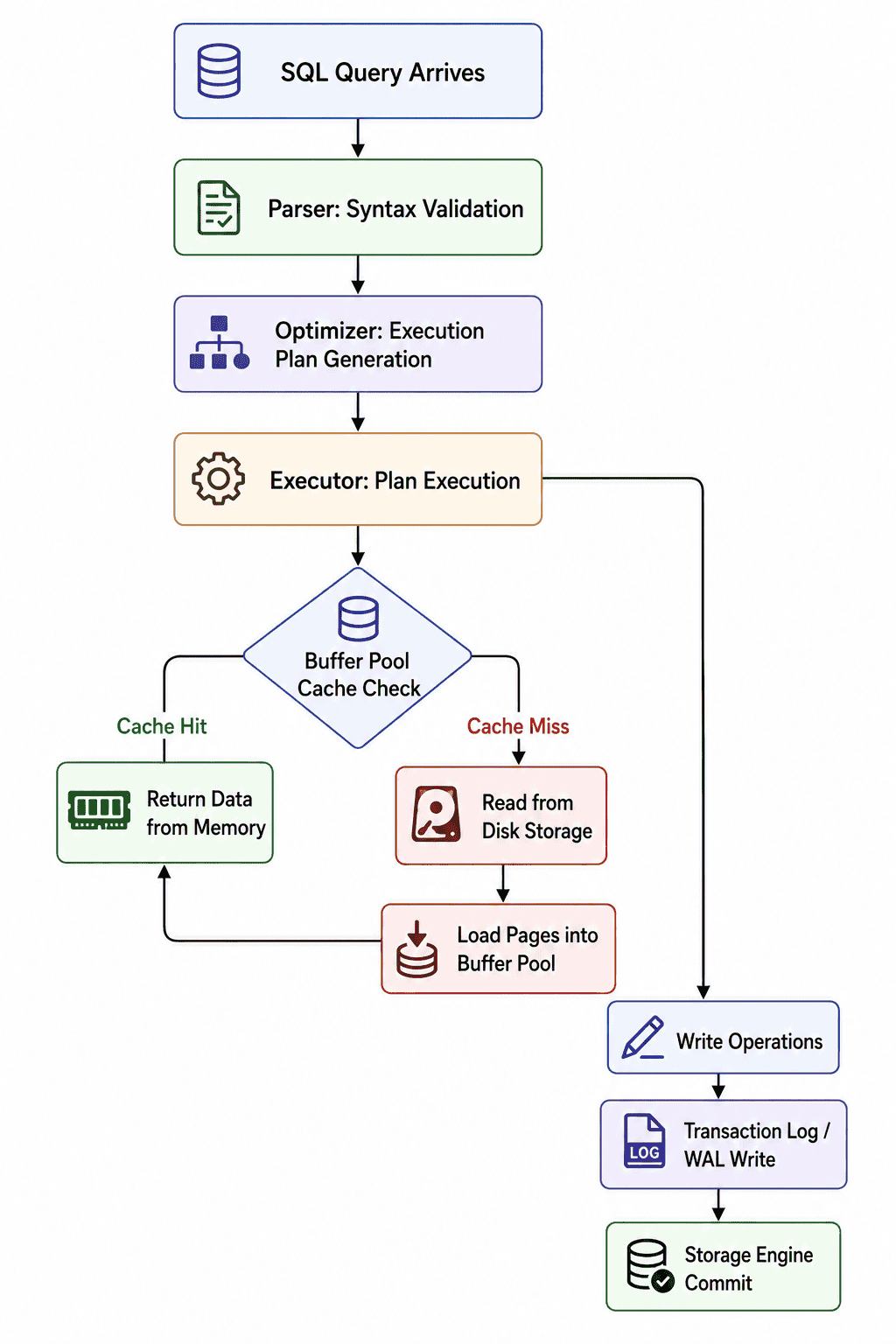
These components don't fail independently. A stale-statistics problem in the optimizer generates a sequential scan that blows through the buffer pool, which triggers disk I/O that competes with transaction log writes. That cascading relationship is why ACID guarantees, and the concurrency models that enforce them, are the next piece of the diagnostic picture.
Transactions, concurrency, and where latency actually hides
ACID compliance carries a performance cost that's worth knowing precisely. Atomicity requires rollback capability, which means WAL writes on every transaction. Isolation causes either lock contention or MVCC overhead depending on your concurrency model. Durability requires an fsync to disk on commit , which is why setting synchronous_commit = off in PostgreSQL yields measurable write throughput gains at the cost of potential data loss on a hard crash. The exposure window is bounded by wal\_writer\_delay (default 200ms), acceptable for high-volume event logging or session stores, but not for financial records or any data where loss of the most recent fraction of a second is unacceptable. MySQL offers an equivalent trade-off with innodb\_flush\_log\_at\_trx_commit = 2 , which flushes the redo log to the OS buffer once per second rather than on every commit, with a similar sub-second data loss window on crash.
PostgreSQL and MySQL InnoDB both use Multi-Version Concurrency Control (MVCC) , where readers get a consistent snapshot of data as of their transaction start time and writers create new row versions rather than overwriting in place. This version separation eliminates the classic reader-blocks-writer contention that predates MVCC adoption.
MVCC's trade-off is dead tuple accumulation. Every UPDATE or DELETE leaves behind an old row version that remains visible to concurrent transactions until no active snapshot references it. On high-churn tables, dead tuples accumulate and bloat table size, degrading sequential scan performance and reducing buffer pool cache efficiency. PostgreSQL's autovacuum process reclaims dead tuples, but the default autovacuum\_vacuum\_scale_factor of 0.2 means vacuuming triggers only after 20% of the table has changed. That is too late for tables receiving millions of updates per day. On high-churn tables, lowering this to 0.01-0.05 and reducing autovacuum\_vacuum\_threshold keeps bloat in check. MySQL handles the same problem through its purge thread, which reclaims old row versions from the undo log. The purge thread runs automatically, but on write-heavy MySQL instances a growing "History list length" in SHOW ENGINE INNODB STATUS signals that purging is falling behind.
SQL Server defaults to pessimistic row-level locking under READ COMMITTED isolation, where readers and writers compete for the same row-level locks. Enabling Read Committed Snapshot Isolation (RCSI) changes this locking behavior to a version-store model aligned with MVCC, allowing readers to proceed against the last committed row version. On databases carrying mixed OLTP and reporting workloads on the same tables, enabling RCSI typically reduces reader-writer lock wait counts, though the trade-off is additional tempdb write pressure on write-heavy workloads.
Deadlocks deserve specific attention because they almost always surface as application-layer errors. When Thread A holds a lock on Row 1 and waits for Row 2 while Thread B holds Row 2 and waits for Row 1, the database detects the cycle and kills one transaction. The application receives ERROR 1213: Deadlock found when trying to get lock; try restarting transaction in MySQL, but depending on your APM tool, the stack trace may point at the application code layer rather than identifying the underlying lock ordering issue. Teams regularly invest time debugging application logic for an issue rooted in transaction ordering and isolation level configuration.
Long-running transactions compound lock contention at scale. A batch job that opens a transaction, processes 50,000 rows, and holds row-level locks for 90 seconds blocks concurrent OLTP writes on those same rows for the entire duration. Those writes don't fail immediately. They queue behind the lock wait timeout, which means your connection pool fills with waiting threads and your application starts returning errors (often HTTP 503s at the load balancer) while the underlying database lock wait may not surface as an explicit error in your application logs.
SQL use cases and what they demand architecturally
OLTP workloads (e-commerce order processing, SaaS user event recording) generate thousands of short, indexed reads and writes per second. The architectural demands are specific: indexes on every column appearing in WHERE clauses and JOIN conditions, connection pooling via PgBouncer or ProxySQL to prevent max_connections exhaustion, and disciplined index hygiene because each index on a high-write table adds overhead to every INSERT and UPDATE . A table receiving 5,000 inserts per minute with seven indexes pays for all seven index updates on each insert. Index proliferation on write-heavy tables is a common source of write latency in systems that grew organically.
When using PgBouncer for OLTP connection pooling, transaction pooling mode is the correct choice. It returns connections to the pool after each transaction completes, giving real connection budget relief. The default session pooling mode holds a connection for the entire client session, which provides no improvement over direct connections. The trade-off: transaction mode is incompatible with server-side prepared statements ( PREPARE / EXECUTE ), so applications relying on those must either switch to client-side preparation or accept session mode's limitations.
Analytics and reporting queries create the opposite pressure. A GROUP BY aggregation across 200 million rows, or a JOIN between a fact table and three dimension tables, produces a query plan that can run for minutes on OLTP-class hardware. Running those analytics queries directly against production tables causes full table scans that compete with concurrent OLTP traffic for buffer pool pages, evicting frequently-accessed data and degrading cache hit ratios across the entire workload. Read replicas and materialized views solve this contention architecturally. A materialized view pre-computes the aggregation, and the analytics query hits the view. PostgreSQL's REFRESH MATERIALIZED VIEW CONCURRENTLY allows refreshes without blocking concurrent reads on the view. Note: CONCURRENTLY requires a unique index on the materialized view; without one, the command raises an error.
SQL also works as an operational monitoring tool, and two query patterns are worth running on production databases as part of your reliability workflow.
For daily active user counts:
SELECT DATE(created_at) AS day, COUNT(DISTINCT user_id) AS dau
FROM events
WHERE created_at >= NOW() - INTERVAL '30 days'
GROUP BY DATE(created_at)
ORDER BY day DESC;
For data quality checks to surface duplicate key inserts (a non-zero duplicate_count signals a data integrity issue worth investigating before it compounds):
SELECT
  COUNT(*) AS total_rows,
  COUNT(DISTINCT id) AS distinct_ids,
  COUNT(*) - COUNT(DISTINCT id) AS duplicate_count
  FROM orders
  WHERE created_at >= NOW() - INTERVAL '1 day';
Both queries run fast on indexed columns and surface problems that threshold-based metric alerts often miss entirely.
Cloud-native SQL deployments on AWS RDS, Azure SQL, and Google Cloud SQL handle storage provisioning and automated backups. High-availability replication and failover are also managed, though traditional log shipping is not a native managed feature on RDS or Cloud SQL. Query performance, connection pool sizing, and instance class selection remain your responsibility. An RDS db.t3.medium instance (4GB RAM) caps max_connections around 450, derived from the formula LEAST({DBInstanceClassMemory/9531392},5000) . If your application opens pools of 50 threads per app server and you run 10 app servers, you've consumed the entire connection budget with a single application tier, before any background jobs or admin connections are counted.
Each of these workload patterns produces a distinct failure signature. The metrics in the next section tell you which pattern you're dealing with.
The SQL performance metrics that tell you something is wrong
Five metric categories give complete signal coverage across the query processing pipeline.
Track query execution time per query pattern, not as a single aggregate. Establish a p95 baseline over a two-week window and alert on any query that crosses 2x its individual baseline. The sources differ by platform: the MySQL slow query log (configured with long\_query\_time = 1 ), pg\_stat\_statements for cumulative PostgreSQL execution stats, and sys.dm\_exec\_query_stats cross-applied to sys.dm\_exec\_sql_text for SQL Server.
Buffer cache hit ratio should stay above 95% for OLTP workloads (Microsoft's stated threshold for SQL Server), though PostgreSQL-specific guidance often targets 99% for hot-data-heavy deployments. A drop below 90% signals insufficient memory, a cold-cache scenario after a server restart, or data growth that has pushed your working set past buffer pool capacity. In PostgreSQL, pg\_statio\_user_tables gives you heap\_blks\_hit and heap\_blks\_read per table so you can identify exactly which tables are generating disk reads. sys.dm\_os\_buffer_descriptors in SQL Server provides equivalent visibility at the buffer pool level.
Lock waits and deadlock counts belong in your alerting baseline. Any non-zero deadlock count in a 5-minute window warrants investigation. In PostgreSQL, pg\_stat\_activity WHERE wait\_event\_type = 'Lock' surfaces currently blocked sessions. In SQL Server, sys.dm\_os\_wait_stats filtered on LCK_ wait types identifies the same condition.
Sustained connection usage above 80% of max_connections is the threshold to act on. It means connection pooling is overdue or undersized. In PostgreSQL, query pg\_stat\_activity for a live connection count. In MySQL, SHOW STATUS LIKE 'Threads_connected' gives the same number.
Wait statistics in SQL Server provide an effective starting point for identifying the resource bottleneck class before you commit to deeper investigation. sys.dm\_os\_wait_stats categorizes accumulated wait time by type: CPU waits ( SOS\_SCHEDULER\_YIELD ), I/O waits ( PAGEIOLATCH_* ), lock waits ( LCK\_M\_* ), and memory waits ( RESOURCE_SEMAPHORE ).
Knowing whether you're I/O-bound or CPU-bound changes your next diagnostic step entirely. These metrics tell you something changed; the observability stack in the next section tells you why.
Building a SQL observability stack: from metrics to root cause
Monitoring alerts on threshold breaches; observability explains why they were breached. That explanation requires three signal layers working together: metrics (query latency, cache hit rate, connection count), logs (slow query logs, error logs, deadlock graphs), and traces (which upstream service triggered the query). When these layers live in separate tools, you spend the incident correlating timestamps instead of diagnosing the problem.
EXPLAIN ANALYZE is the hands-on diagnostic for any slow query. A query against a large users table running at 800ms average might look like this:
EXPLAIN ANALYZE
SELECT * FROM users
WHERE account_status = 'active'
AND last_login < NOW() - INTERVAL '90 days';
A plan showing Seq Scan on users (cost=0.00..45231.00 rows=2847182 width=...) (actual time=0.031..823.400 rows=2841000 loops=1) tells you the query is scanning every row. Reading the plan output:
cost=0.00..45231.00: the planner's estimated startup and total cost in arbitrary units (useful for comparing alternative plans, not as absolute time)rows=2847182: the planner's row estimate; compare againstactual rowsto detect stale statisticsactual time=0.031..823.400: real execution time in milliseconds for the first row and last row- The dominant node is the one with the highest
actual timespread. That's where optimization effort should focus
Important: When running EXPLAIN ANALYZE on INSERT , UPDATE , or DELETE statements, always wrap the call in a transaction and roll back. EXPLAIN ANALYZE actually executes the statement, so without the rollback you'll modify live data.
Adding a composite index changes the plan:
CREATE INDEX idx_users_status_login ON users(account_status, last_login);After the index exists, EXPLAIN ANALYZE returns Index Scan using idx\_users\_status_login with dramatically lower row estimates and actual execution time orders of magnitude faster than the sequential scan. The index changed the access pattern from O(n) to O(log n) with no schema changes required. Reading the plan before tuning the query applies across PostgreSQL and MySQL ( EXPLAIN ANALYZE FORMAT=TREE in MySQL 8.0+ provides equivalent detail including actual execution timing; EXPLAIN FORMAT=JSON gives plan structure but not runtime metrics).
Platforms like ManageEngine Applications Manager address the correlation problem by co-locating database metrics with APM data, eliminating the timestamp cross-referencing that fragmented tooling requires. The integrated APM and database views let you correlate query spikes with downstream API latency without switching platforms.
Three troubleshooting scenarios: symptom to resolution
These scenarios map observed symptoms to specific diagnostic queries and resolution paths, drawing on SQL Server performance monitoring best practices documented by Paessler.
Each scenario traces back to one of the architectural components covered earlier: Scenario A targets the buffer pool, Scenario B exposes transaction and lock contention, and Scenario C surfaces query optimizer issues. The ordering follows the diagnostic sequence most teams encounter: cache degradation first, then concurrency bottlenecks, then plan regression after a code change.
Scenario A: Buffer cache hit ratio drops from 98% to 87% overnight
Query pg\_statio\_user_tables for tables with elevated heap\_blks\_read relative to heap\_blks\_hit :
SELECT relname, heap_blks_read, heap_blks_hit,
  ROUND(100.0 * heap_blks_hit / NULLIF(heap_blks_hit + heap_blks_read, 0), 2) AS hit_ratio
FROM pg_statio_user_tables
ORDER BY heap_blks_read DESC
LIMIT 1
Tables with low hit ratios are generating disk reads. Cross-reference with pg\_stat\_statements to find queries with elevated blks_read that appeared after your last deployment. Common causes include a new query doing a full sequential scan on a large table, data growth pushing the working set past shared_buffers , or a missing index introduced by a schema migration. If a recently deployed query is the culprit, add a covering index. If data growth is the driver, increase shared_buffers to 25-30% of available system RAM ( PostgreSQL's guideline for dedicated database hosts ), remembering that this requires a service restart and that you should update effective\_cache\_size at the same time.
Scenario B: Application returns lock wait timeout errors during peak traffic
On SQL Server, query sys.dm\_exec\_requests filtered on blocking\_session\_id IS NOT NULL to identify blocking session SPIDs directly. Use sys.dm\_os\_wait_stats filtered on LCK\_M\_ wait types to confirm the lock wait type distribution. On PostgreSQL, run:
SELECT pid, wait_event_type, wait_event, query, state, query_start
FROM pg_stat_activity
WHERE wait_event_type = 'Lock'
ORDER BY query_start;
Find the session holding the lock the waiting sessions need and check its query_start time. A transaction open for 45 minutes during a window where your batch job runs for 5 minutes points to an uncommitted batch transaction holding row-level locks against OLTP traffic. The resolution is isolating batch processing to a maintenance window or, on SQL Server, enabling RCSI so readers proceed against the version store while writers continue updating live rows concurrently.
Scenario C: Query p95 latency doubles after a deployment
On SQL Server, check for parameter sniffing . The optimizer caches an execution plan on first execution using the specific parameter values passed at that moment. If those values don't represent the full distribution, every subsequent call runs the suboptimal cached plan:
SELECT TOP 10
  qs.total_elapsed_time / qs.execution_count AS avg_elapsed_us,
  qs.execution_count,
  SUBSTRING(qt.text, (qs.statement_start_offset/2)+1,
    ((CASE qs.statement_end_offset
      WHEN -1 THEN DATALENGTH(qt.text)
      ELSE qs.statement_end_offset END
    - qs.statement_start_offset)/2)+1) AS query_text
FROM sys.dm_exec_query_stats qs
CROSS APPLY sys.dm_exec_sql_text(qs.sql_handle) qt
ORDER BY avg_elapsed_us DESC;
Use sys.dm\_exec\_query_plan to retrieve the cached plan and compare it against the output from running the same query with OPTION (RECOMPILE) to confirm sniffing is the root cause. Once confirmed, your remediation options are:
- Immediate incident mitigation:
DBCC FREEPROCCACHE(plan_handle)to evict the bad plan, forcing recompilation on the next call - Permanent per-query fix: Add
OPTION (RECOMPILE)as a query hint, which forces a fresh plan on every execution (at the cost of compilation overhead per call) - Plan stability alternative:
OPTION (OPTIMIZE FOR UNKNOWN)directs the optimizer to use average distribution statistics rather than the first-call parameter values, avoiding the worst-case skew without per-execution recompile cost
On PostgreSQL, a post-deployment spike often points to stale planner statistics. Running ANALYZE tablename after a large data load forces the planner to update its row count estimates, and the optimizer picks a correct plan the next time the query runs.
Your instrumentation starting point: do this today
These three commands give you immediate slow-query visibility with no external tooling required. Think of them as the triage step: they identify which queries to investigate. The follow-on diagnostic is EXPLAIN ANALYZE (covered in the Observability section above), which tells you why those queries are slow.
For PostgreSQL, enable pg\_stat\_statements by adding shared\_preload\_libraries = 'pg\_stat\_statements' to postgresql.conf and restarting. Then run:
SELECT query, calls,
  total_exec_time / calls AS avg_ms,
  rows
FROM pg_stat_statements
ORDER BY avg_ms DESC
LIMIT 10;
This returns your top 10 slowest queries by average execution time, with call counts so you can prioritize by total impact (high avg_ms combined with high call count) rather than worst single execution. Note: total\_exec\_time is available in PostgreSQL 13+. On PostgreSQL 12 and earlier, substitute total_time .
For MySQL, set slow_query_log = ON and long_query_time = 1 in my.cnf , then run:
mysqldumpslow -s t /var/log/mysql/mysql-slow.log
The -s t flag sorts by total execution time, weighting high-frequency moderate-latency queries above rare but slow outliers. That sort order gives you the highest-impact targets first.
For SQL Server, no configuration changes are required. Run directly against the DMVs:
SELECT TOP 10
  total_elapsed_time / execution_count AS avg_elapsed_us,
  execution_count,
  total_elapsed_time,
  qt.text
FROM sys.dm_exec_query_stats
CROSS APPLY sys.dm_exec_sql_text(sql_handle) qt
ORDER BY avg_elapsed_us DESC;